Natural Language Processing : How do machines make sense of questions ?
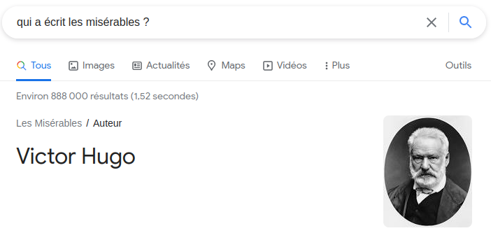
When searching for specific information in large volumes of text, we tend to use key words: For example, in a text about French literature, if we are looking for the name of the author of les Misérables, we can search within this text for terms that are likely to be close to the answer we are looking for: Misérables auteur “ or “Misérables écrivain “.
But some search engines are able to interpret questions asked in natural language. For example, if one types into the Google search bar “Who wrote Les Misérables?”, the algorithm is able to detect that the entity searched for is an author, without the word “author” being explicitly present:
How do these algorithms capture the meaning of a question, and what kind of information is being sought? We propose here to build a program with the following goal: For a given question, we want to find out what entity is being sought (a place? a time? a distance? a person?)
A naive approach: building lexical fields by hand
The first idea that could come to mind would be to define rules based on the lexical fields of the words in the question: for example, if the question contains one of the declensions of the verbs “to write”, “to draft”, it is likely to be about an author. How to generalize this idea and propose a lexical field for each category of question?
The first step is to clearly define the categories in which the questions will be classified. To do this, we can use existing categories.
We will use here a pre-existing dataset containing 5452 questions, the [TREC] database (https://search.r-project.org/CRAN/refmans/textdata/html/dataset_trec.html), for Text REtrieval Conference. Each question, in English, is classified among 6 categories (Abbreviation, Description and abstract concepts, Entities, Human beings, Locations and Numeric values) and 50 subcategories, of which we can find the details here
Let’s first look at what our dataset looks like:
#We extract the table from the csv file using the pandas library
import pandas as pd
data = pd.read_csv('/media/tidiane/D:/Dev/NLP/data/Question_Classification_Dataset.csv', encoding='latin-1')
data
| Questions | Category0 | Category1 | Category2 | |
|---|---|---|---|---|
| 0 | How did serfdom develop in and then leave Russ… | DESCRIPTION | DESC | manner |
| 1 | What films featured the character Popeye Doyle ? | ENTITY | ENTY | cremat |
| … | … | … | … | … |
| 5447 | What ‘s the shape of a camel ‘s spine ? | ENTITY | ENTY | other |
| 5448 | What type of currency is used in China ? | ENTITY | ENTY | currency |
| 5449 | What is the temperature today ? | NUMERIC | NUM | temp |
| 5450 | What is the temperature for cooking ? | NUMERIC | NUM | temp |
| 5451 | What currency is used in Australia ? | ENTITY | ENTY | currency |
In each category, we can see which words are the most used: These are the most likely to form a coherent lexical field.
#We group the questions by category 2:
data_group = data.groupby(['Category2'])['Questions'].apply(lambda x: ' '.join(x)).reset_index()
#We then transform our aggregated questions into a dictionary containing the frequency of each word:
def word_count(str):
counts = dict()
words = str.split()
for word in words:
if word in counts:
counts[word] += 1
else:
counts[word] = 1
counts = dict(sorted(counts.items(), key=lambda item: item[1], reverse=True))
return counts
data_group['count'] = data_group['Questions'].apply(word_count)
# Finally, the 10 most frequent words in each category are displayed:
for i in range(len(data_group)) :
print(data_group.loc[i, "Category2"])
count = data_group.loc[i, "count"]
print(list(count.keys())[0:10], "\n")
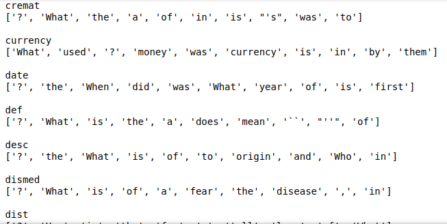
The 10 most frequently occurring terms in each category
Taking advantage of word frequency: the use of bayesian inference
From these created lexical fields, we will build a question classifier, based on the Bayesian method. The idea is simple: we will calculate the probabilities of belonging to each category for each word and then generalise these probabilities to the sentence level.
Let’s imagine for the moment that our database consists of only 3 questions, each in a different category:
–How many departments are there in France ? (count)
–Who is the current french president ? (ind)
–When did french people rebel against their king ? (date)
First, we will list the frequency of occurrence of each term in each category:
| count | ind | date | |
|---|---|---|---|
| against | 0 | 0 | 1 |
| are | 1 | 0 | 0 |
| current | 0 | 1 | 0 |
| departments | 1 | 0 | 0 |
| did | 0 | 0 | 1 |
| France | 1 | 0 | 0 |
| french | 0 | 1 | 1 |
| How | 1 | 0 | 0 |
| in | 1 | 0 | 0 |
| is | 0 | 1 | 0 |
| king | 0 | 0 | 1 |
| many | 1 | 0 | 0 |
| people | 0 | 0 | 1 |
| president | 0 | 1 | 0 |
| rebel | 0 | 0 | 1 |
| the | 0 | 1 | 0 |
| their | 0 | 0 | 1 |
| there | 1 | 0 | 0 |
| When | 0 | 0 | 1 |
| Who | 0 | 1 | 0 |
Here is a 4th sentence: How many people live in France ?
Can we tell from our three previous sentences to which category this one belongs ?
For example, let’s try to calculate the probability that our sentence belongs to the count category, knowing that it contains the words “How many people are in France”. We will note this probability $P(count/”How\ many\ people\ are\ in\ France”)$
The Bayes’ theorem allows us to write the following equation:
$P(count/”How\ many\ people\ are\ in\ France”) = \frac{P(“How\ many\ people\ are\ in\ France”/count) * P(count)}{P(“How\ many\ people\ are\ in\ France”)} $
How to calculate the probability $P(“How\ many\ people\ are\ in\ France”/count)$, i.e. the probability of coming across this exact sentence when a sentence in the count category is drawn at random?
Our data set is far too small to obtain this probability directly. We then make the simplifying assumption that the individual occurrences of the words are independent events. We can then decompose the probability as follows:
$P(“How\ many\ people\ are\ in\ France”/count) = P(“How”/count) * P(“many”/count) * P(“people”/count) * P(“are”/count) * P(“in”/count) * P(“France”/count)$
Let us now look at each of these expressions : $P(“How”/count)$ expresses the probability of encountering the word “How” in a question of category count. Now, this word appears 1 time in the category, which has a total of 7 words (we can refer to the table presented above): $P(“How”/count) = 1/7$
The word “many” also appears once : $P(“many”/count) = 1/7$
The word “people” does not appear in the count category. Words outside the category will have an arbitrarily small but non-zero probability associated with them, to prevent the final product from falling to zero. $P(“many”/count) = 10^{⁻3}$
After calculating the probability of occurrence of each word, we obtain by their product the term $P(“How\ many\ people\ are\ in\ France”/count)$. Il est égal à $(1/7)⁵ * 10^{⁻3} \approx 5,94 * 10^{⁻8}$
The same way, $P(“How\ many\ people\ are\ in\ France”/ind)= {10^{⁻3}}^6 = 10^{⁻18} $
Finally, $P(“How\ many\ people\ are\ in\ France”/date)= 1/7 * {10^{⁻3}}^5 \approx 1,42 * 10^{⁻16} $
It can be noted that the calculated probabilities are directly dependent on the number of sentence terms present in each category: 5 out of 6 words in the sentence are present in the count category, compared to 0 in ind and 1 in date.
We can then notice that the probabilities $P(count)$, $P(date)$ and $P(ind)$ are all equal to $1/3$.
Dans l’expression $\frac{P(“How\ many\ people\ are\ in\ France”/ \textbf {categorie}) * P(\textbf {categorie})}{P(“How\ many\ people\ are\ in\ France”)} $, The only non-constant term is the one we have just calculated. It is thus him who will determine the order of our probabilities : $P(count/”How\ many\ people\ are\ in\ France”) > P(date/”How\ many\ people\ are\ in\ France”) > P(ind/”How\ many\ people\ are\ in\ France”)$
Our initial sentence is therefore, according to our model, more likely to belong to the count category.
It is this idea of Bayesian inference that we will use to build our classifier, this time taking all the sentences in our database TREC. We hope that the diversity of the sentences present in this database will contribute to the robustness of our model.
Putting theory into practice : Building a Bayesian classifier
We will divide our question base in two. One part will be used to train our model, and the other to evaluate its performance. This is a common practice which avoids evaluating a model on a sentence on which it has been trained, which would bias our results.
#We import from the sklearn library some useful functions for word counting.
from sklearn import feature_extraction, model_selection, naive_bayes, pipeline, manifold, preprocessing,feature_selection, metric
#We split our base in two
dtf_train, dtf_test = model_selection.train_test_split(data, test_size=0.3)
y_train = dtf_train["Category2"].values
corpus = dtf_train["Questions"] #set of texts for practice questions
#We create our table of occurrence of words in each category
vectorizer = feature_extraction.text.CountVectorizer(max_features=10000)#, ngram_range=(1,1))
vectorizer.fit(corpus)
classifier = naive_bayes.MultinomialNB()
X_train = vectorizer.transform(corpus)
model = pipeline.Pipeline([("vectorizer", vectorizer),
("classifier", classifier)])## train classifier
model["classifier"].fit(X_train, y_train)
X_test = dtf_test["Questions"].values
y_test = dtf_test["Category2"].values
predicted = model.predict(X_test)
predicted_prob = model.predict_proba(X_test)
metrics.accuracy_score(y_test, predicted) #0.4902200488997555
Our classifier has a correct answer rate of about 49%, which is quite low. However, we have to put this result in perspective with the fact that we have 50 categories: pure chance would give us a success rate of only 2%.
For class 1, which has only 6 categories, the accuracy is 48.5%.
An approach taking into account the structure of the language: word vectors
Our Bayesian model, if it does better than pure chance, has an inherent disadvantage: Each occurrence of a word is considered as independent of the others.
However, some words have a semantic proximity: different conjugations of the same verb, or place names, for example. This proximity is not modeled by our approach, which considers words as variables that have no relation between them.
The concept of embedding makes each word correspond to a point in a continuous space, usually multidimensional.
Here is an example of embeddings of 34 words, in two dimensions:
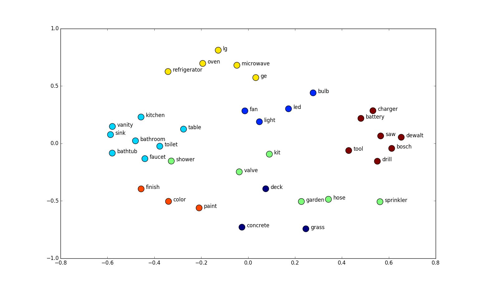
We notice that words with similar meaning are often next to each other, and that they even form coherent semantic groups. And this is precisely why this method is interesting: it allows to represent the structure of the language used, and to facilitate the task of some language processing algorithms.
But then, how to produce embeddings? Most methods exploit existing text corpora. The basic assumption of these methods is that words that appear frequently in similar word neighborhoods are more likely to share attributes. For example, words appearing after a personal pronoun are more likely to be verbs, words belonging to the same lexical field are more likely to be next to each other, etc…
We will try to build our own embeddings, following the Continuous bag-of-words (CBOW) method, proposed by Mikolov. This method consists in training a neural network with a hidden layer to predict a word from its neighbors.
To do this, we will exploit our database of questions. Our network will take as input a word from a question, and it will have to correctly predict a word from its neighborhood.
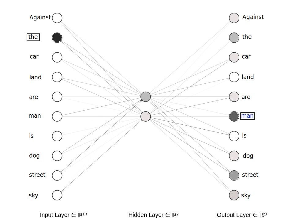
A simplified version of the model has been put above. We have in input the word “the”: in the input layer, the neuron corresponding to this word is activated. We will train the network to predict a neighboring word, here the word “man”.
At the end of the training, we hope that words with similar meanings will lead to the same predictions of neighboring words, and will therefore have similar hidden layer activations: it is these activation values that we will consider later as our embeddings.
We first adapt our dataset to be readable by the network: we will create pairs of words $(x,y)$, $y$ being the word to predict, and $x$ a “neighbor” word. We consider here as a neighbor word of $y$ any word appearing in the same sentence and distant of 4 words at most.
import itertools
import pandas as pd
import numpy as np
import re
import os
from tqdm import tqdm
# Drawing the embeddings
import matplotlib.pyplot as plt
# Deep learning:
from keras.models import Input, Model
from keras.layers import Dense
from scipy import sparse
texts = [x for x in data['Questions']]
# Defining the window for context
window = 4
import re
import numpy as np
def text_preprocessing(
text:list,
punctuations = r'''!()-[]{};:'"\,<>./?@#$%^&*_“~''',
stop_words = [ "a", "the" , "to" ]
)->list:
"""
A method to preproces text
"""
for x in text.lower():
if x in punctuations:
text = text.replace(x, "")
# Removing words that have numbers in them
text = re.sub(r'\w*\d\w*', '', text)
# Removing digits
text = re.sub(r'[0-9]+', '', text)
# Cleaning the whitespaces
text = re.sub(r'\s+', ' ', text).strip()
# Setting every word to lower
text = text.lower()
# Converting all our text to a list
text = text.split(' ')
# Droping empty strings
text = [x for x in text if x!='']
# Droping stop words
text = [x for x in text if x not in stop_words]
return text
def word_count(str):
counts = dict()
words = str.split()
for word in words:
if word in counts:
counts[word] += 1
else:
counts[word] = 1
return counts
word_lists = []
all_text = []
for text in texts:
# Cleaning the text
text = text_preprocessing(text)
# Appending to the all text list
all_text += text
# Creating a context dictionary
for i, word in enumerate(text):
for w in range(window):
# Getting the context that is ahead by *window* words
if i + 1 + w < len(text):
word_lists.append([word] + [text[(i + 1 + w)]])
# Getting the context that is behind by *window* words
if i - w - 1 >= 0:
word_lists.append([word] + [text[(i - w - 1)]])
frequencies = {}
for item in all_text:
if item in frequencies:
frequencies[item] += 1
else:
frequencies[item] = 1
word_lists is a list of pairs (neighboring word, word to predict) found in the text. It removes the words that are too uncommon, likely to disturb the performance of the model:
word_lists = [item for item in word_lists if frequencies[item[0]]>20 and frequencies[item[1]]>20]
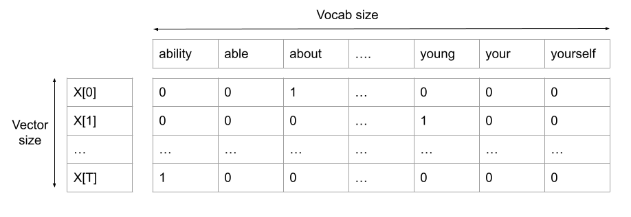
We will then create two vectors, X and Y, containing respectively the list of neighboring words and the words to predict, encoded in one-hot form. This means that each vector is of size N (= size of the total vocabulary) and contains a 1 at the position corresponding to the coded word, the rest of the vector being zero.
dict_short = {}
j = 0
for i, word in enumerate(word_lists):
if word[0] not in dict_short :
dict_short.update({ word[0]: j })
j=j+1
n_words_short = len(dict_short)
# Creating the X and Y matrices using one hot encoding
X = []
Y = []
words = list(dict_short.keys())
for i, word_list in tqdm(enumerate(word_lists)):
# Getting the indices
main_word_index = dict_short.get(word_list[0])
context_word_index = dict_short.get(word_list[1])
# Creating the placeholders
X_row = np.zeros(n_words_short)
Y_row = np.zeros(n_words_short)
# One hot encoding the main word
X_row[main_word_index] = 1
# One hot encoding the Y matrix words
Y_row[context_word_index] = 1
# Appending to the main matrices
X.append(X_row)
Y.append(Y_row)
The format of the X and Y objects now allows us to train a neural network:
import tensorflow as tf
model = tf.keras.Sequential([
tf.keras.layers.Dense(2, activation='softmax'),
tf.keras.layers.Dense( n_words_short) #(len(unique_word_dict))
])
model.compile(loss = 'categorical_crossentropy', optimizer = 'adam')
model.fit(x=np.array(X), y=np.array(Y), epochs=10)
On peut maintenant visualiser nos embeddings en 2 dimensions :
import random
weights = model.get_weights()[0]
# Creating a dictionary to store the embeddings in. The key is a unique word and
# the value is the numeric vector
embedding_dict = {}
for word in words:
embedding_dict.update({
word: weights[dict_short.get(word)]
})
# Ploting the embeddings
plt.figure(figsize=(10, 10))
for word in list(dict_short.keys()):
coord = embedding_dict.get(word)
plt.scatter(coord[0], coord[1])
plt.annotate(word, (coord[0], coord[1]))
We can notice that several related words are relatively close (dog/animal, day/year, city/capital). But it is difficult to find a global consistency.
We can also create higher dimensional embeddings: For that, we have to change the size of the hidden layer of our network. A higher dimension of embeddings allows the network to form more complex semantic structures between the different words. Here are some embeddings trained on the same text, but in 3 dimensions:
Here again, we notice similarities between close words. We will try to use our embedding structure to classify our questions.
Using word vectors for our classification
In the same spirit as word embeddings, several works are looking at sentence embeddings, and the possibility of capturing their meaning through vectors. Arora et al. describe several methods to create these sentence embeddings, but also point out that the method consisting in taking the average of the word embeddings of the sentence gives satisfactory results. This is what we will try here:
def sentence_mean(sentence):
array_vect = [np.array([0,0,0])]
for i in range(len(sentence)):
if sentence[i] in embedding_dict.keys():
array_vect.append(embedding_dict[sentence[i]])
return np.array(sum(array_vect)/max(1,len(array_vect)))
from nltk.tokenize import word_tokenize
data['processed_text'] = data["Questions"].str.lower().replace(r"[^a-zA-Z ]+", "")
data['vec'] = data['processed_text'].apply(lambda x: word_tokenize(x))
data['mean_vec'] = data['vec'].apply(lambda x: sentence_mean(x))
data['x'] = data['mean_vec'].apply(lambda x: x[0])
data['y'] = data['mean_vec'].apply(lambda x: x[1])
data['z'] = data['mean_vec'].apply(lambda x: x[2])
We have associated here to each question the average of the 3d embeddings of the words which compose it. We can therefore associate a point to each sentence on a graph:
We have also displayed the categories of the questions, with different colors. It would be unreadable to display all 50 subcategories, so we show the 6 first level categories (Abbreviation, Description and abstract concepts, Entities, Human beings, Locations and Numeric values).
There is no marked separation between the categories, but one can already notice clusters of sentences of the same category in some places. If the groups were more marked, it would be easier to classify a sentence according to the group of points to which its embedding belongs.
To refine our classification tool, we will use word embeddings that are more efficient, because they have already been trained on a much larger corpus: the Glove.
These vectors are produced in the same way as explained above, but are of dimension 50, and are trained on the entire English content of wikipedia (2014), a corpus of 1.6 billion words.
import gensim.downloader
glove_model = gensim.downloader.load('glove-wiki-gigaword-50')
def sentence_mean_glove(sentence):
array_vect = []
for i in range(min(4,len(sentence))):
if sentence[i] in glove_model.key_to_index.keys():
array_vect.append(glove_model[sentence[i]])
return sum(array_vect)/len(array_vect)
data['mean_vec_glove'] = data['vec'].apply(lambda x: sentence_mean_glove(x))
Each question is now represented by a vector of size 50. To be able to visualize these vectors, we will reduce their dimensions with the t-sne algorithm :
from sklearn.manifold import TSNE
sentence_vec_tsne = TSNE(n_components=3).fit_transform(data['mean_vec_glove'].tolist())
We can now display our point cloud:
import plotly.graph_objects as go
fig = go.Figure(data=[go.Scatter3d(
x=[a[0] for a in sentence_vec_tsne], # ie [0, 1, 2, 3]
y=[a[1] for a in sentence_vec_tsne], # ie [0, 1, 2, 3]
z=[a[2] for a in sentence_vec_tsne], # ie [0, 1, 2, 3]
hovertemplate='<b>%{text}</b><extra></extra>',
text = data["Questions"],
mode='markers',
marker=dict(
size=3,
opacity=0.8,
color=data['Category1'].map(col_dict),
)
)])
fig.show()
We can notice that the groups are much more marked. We will use these groupings to build a classifier. The principle is simple: For a given question, we will compute its sentence embedding, and associate it with the class of the closest known question:
X = data['mean_vec_glove'].tolist()
y = data['Category2'].tolist()
from sklearn.model_selection import train_test_split
X_train, X_test, y_train, y_test = train_test_split(X, y, test_size=.4, random_state=42)
from sklearn.neighbors import KNeighborsClassifier
neigh = KNeighborsClassifier(n_neighbors=1)
neigh.fit(X_train, y_train)
score = neigh.score(X_test, y_test)
score
The classification score is this time 0.675 for class 1 (6 categories), and 0.567 for class 2 (50 categories). It is still quite low compared to the state of the art in classification, but already higher than our previous method.
We notice that beyond the classification, our embeddings have succeeded in modeling the semantics of our questions: the neighboring sentences have systematically a close meaning. This model could be used as a search engine in domains where the semantics of sentences is important, such as the search for similar questions on a self-help forum.
To further improve our classifier, we could use more sophisticated methods than the average for our embedding sentences: Conneau et al. propose the use of recurrent networks to capture the meaning of the set of embeddings of the words of a sentence, in a similar way to what is done in this article on image description.
Cer et al. propose two methods, one based on convolution, a method which is also discussed here, and the other based on transformers, attention-based networks, which we might discuss about in a future article.
The code used in this article is available here